The chaotic physical pendulum

Thomas Gasenzer

Problems in Theoretical Physics I - Mechanics

Chaotic behaviour of the damped, harmonically driven pendulum

The description given here is based on the book by Gregory L. Baker and J. P. Gollub. Chaotic dynamics: an introduction. Cambridge University Press, 1990.
Even more on the pendulum can be found in a book recently published at the other place: Gregory L. Baker and James A. Blackburn. The Pendulum - A Case Study in Physics. Oxford University Press, 2005.

See also publication on a Demonstration Experiment developed at the University of Heidelberg
by H. Hauptfleisch, T. Gasenzer, K. Meier, O. Nachtmann, and J. Schemmel:
arXiv:0905.2015 [physics.ed-ph] [Abstract, PDF]

Theory

A damped, sinusoidally driven pendulum of mass m (or weight W) and length l is described by the following equation of motion:

mld²/dt² + d/dt + Wsin = Acos(_Dt)

where the left hand terms represent acceleration, damping and gravitation, and the right hand side is the forcing term. In dimensionless form the equation can be rewritten as:

d²/dt² + (1/q)d/dt + sin = gcos(_Dt)

where q is the damping factor, g is the forcing amplitude and _D is the angular forcing frequency. One may rewrite this differential equation as a set of first order coupled equations:

d/dt = -(1/q) - sin + gcos

d/dt =

d/dt = _D

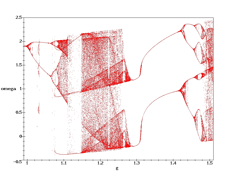
where is the angular frequency, is the angular position, and is the phase of the forcing term. (,,) are the three dynamic variables necessary for chaos and the sin and cos terms provide the nonlinearity. The pendulum displays a variety of ordered and chaotic behaviour depending on the values of the parameters g,_D and q.

For small oscillations the undamped pendulum has a natural angular frequency of unity in the units employed here. Chaotic behaviour arises partly from the interaction between the driving frequency and the natural frequency so we can expect to find interesting behaviour for driving frequencies close to 1.

Phase plots

The pendulum has a 3-dimensional phase space with ,, as the coordinate axes. In the following phase portraits the phase trajectory is projected onto the (,) plane. In this plane periodic motion appears as closed loops.

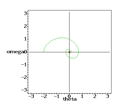
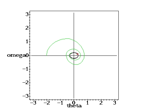
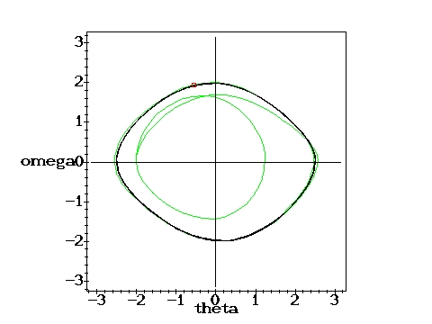
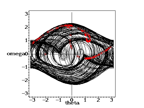
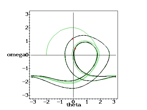
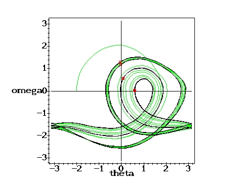
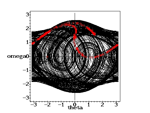
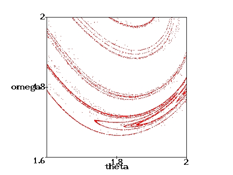
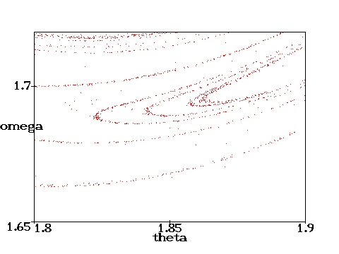
The green part of the trajectories indicates the initial oscillation before the motion becomes periodic. In the chaotic cases, the whole trajectory is plotted in black. The red points represent the Poincare section, which indicates the state of the pendulum after each period of the driving force. It therefore corresponds to a stroboscopic view at the pendulum in the phase plane. For the chaotic cases only a limited number of phase and Poincare points have been calculated. With the time approaching infinity, the corresponding phase plots would become uniformly black within certain regions and the Poincare sections would loose their discreteness.

Without drivin force: Damped oscillator. g=0, q=2, D=0.6667	Low driving force: Periodic motion.g=0.2, q=2, D=0.6667

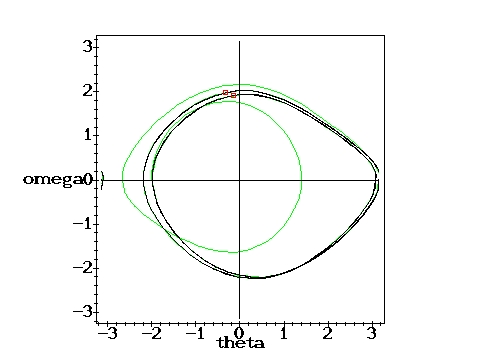
Medium driving force: Single Poincare point.g=0.9, q=2, D=0.6667	Attractor with bifurcation: Two Poincare points.g=1.07, q=2, D=0.6667

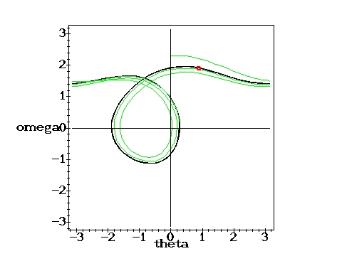
Chaotic state: g=1.15, q=2, D=0.6667	Again periodic, single Poincare point: g=1.35, q=2, D=0.6667

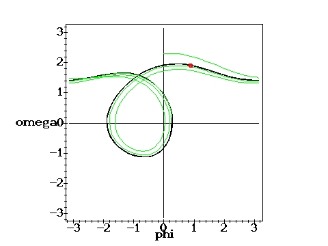Same force, different initial cond.: g=1.35, q=2, D=0.6667	Again a bifurcation: g=1.45, q=2, D=0.6667

Another bifurcation, four Poincare points: g=1.47, q=2, D=0.6667	Again chaotic: g=1.5, q=2, D=0.6667

The Poincare Section

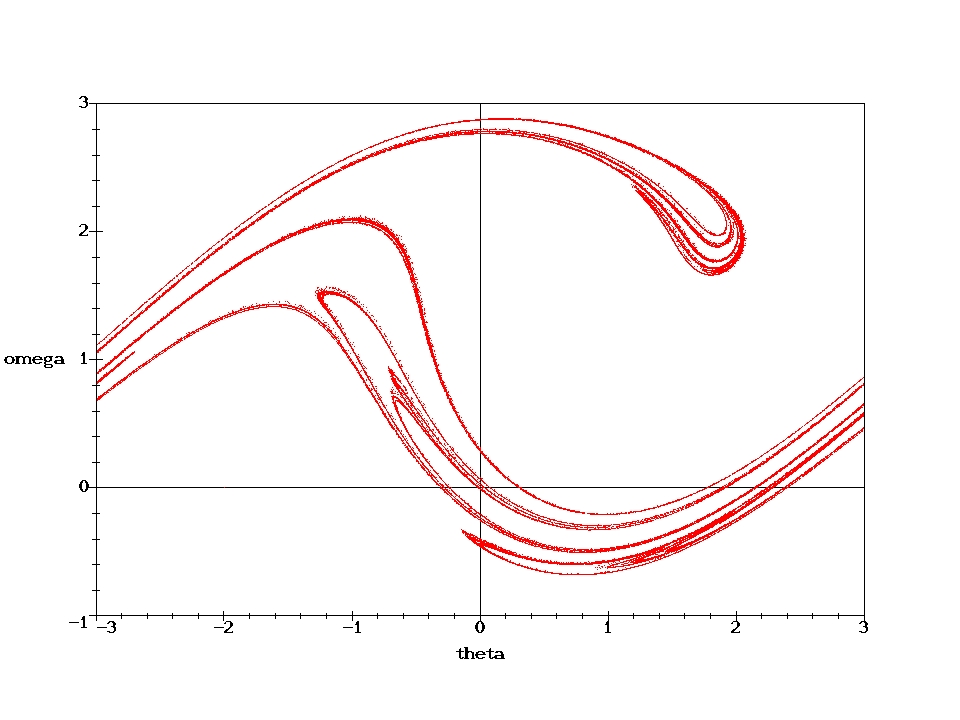
In the following plots (parts of) the Poincare section for the chaotic case with g=1.5, q=4,_D=0.6667 (i.e., with a weaker damping than above) are shown. 100000 cycles have been computed. They nicely illustrate the self similarity of the Poincare section.

The Bifurcation Diagram

The above plots may be better related to each other using the bifurcation diagram, which shows the Poincare section projected onto the omega axes for varying values of g between 1.0 and 1.5. The regions with many irregularly sputtered points correspond to chaotic behaviour of the pendulum. For each g, 50 cycles, i.e. Poincare points have been calculated after an initial number of 100 cycles. This limited number of data points causes the lines to widen around the bifurcations.